Simulating Branch Predictors
Branch predictors are an essential component of modern CPUs as well as the subject of this very silly meme I encountered on The Internet one day:
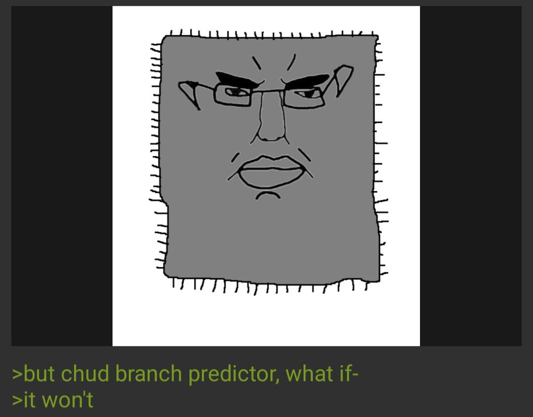
This very silly meme led me down a rabbit hole where I discovered progressively wilder statistics about state-of-the-art branch predictors, like that they…
- are correct over 98% of the time
- are essentially small neural networks embedded in the chip
- look hundreds or even thousands of branches into the past to make decisions
My initial reaction was “how could any of this possibly be true?”.
To find out, I read up some more and coded up a basic simulation. This turned into a protracted effort to implement, run, and probe the structure of increasingly complicated versions of these fascinating devices. The goal of this blog post is to serve as a writeup of this process.
How to build a branch predictor
I will be assuming you have some basic knowledge of computer architecture. Some recommended pre-reading:
- What Every Programmer Should Know about How CPUs Work: Talk by Matt Godbolt; a good primer on relevant aspects of computer architecture
- Branch prediction: Blog post by Dan Luu on branch prediction
- The ITTAGE indirect branch predictor: Blog post by Nelson Elhage on state-of-the-art predictors specifically
Onwards.
Branches
A branch is a control flow statement such as an if-else statement or switch case.
Code that looks like…
 1int main() {
 2    int happy = 1;
 3    int know_it = 1;
 4
 5    if (happy & know_it) {
 6        ClapYourHands();
 7    } else {
 8        ...
 9    }
10}
… appears like this to a computer (not really but it’s a good enough mental model):
1    cmp     r0, #0          ; comparison
2    beq     .LBB0_2         ; jump to else
3    bl      ClapYourHands() ; function call
4    b       .LBB0_3
In human terms:
- Check whether a variable is equal to 0
- If yes, then start reading and executing code located at
.LBB0_2 - Otherwise, start reading and executing code inside the function
ClapYourHands
In a modern pipelined processor, the outcome of the comparison (Step 1) may not be known for several cycles, which leaves you only one of two choices: wait until you know which instruction to read next, or make a guess.
Guessing results in one of two outcomes:
- Correct: The program continues running with zero delay
- Incorrect: The program needs to cancel running the loaded instructions, undo their results, then load the code from the correct branch.
- Implemented correctly, this results in minimal delay over just waiting for the branch to resolve.
Just waiting means you’re guaranteed a delay every time. Thus, the motivation for branch prediction.
The saturating counter
The humble saturating counter is the basic building block of most modern predictors.
Basically it’s an n-bit integer (where n is typically 2 or 3) that can be incremented up to a maximum value, or decremented down to a minimum value.
Concretely, a two-bit saturating counter is much like a chalkboard with enough space to draw 4 tally marks. You can keep adding marks until you fill up the board or erase marks until it’s empty, but that’s as much state as you can store.
We can use this to predict a branch with a two-step algorithm:
- Predict: If the value of the counter is above a certain threshold, predict that the branch will be TAKEN. Otherwise, predict NOT TAKEN.
- Update: Once you learn the outcome of the branch, increment it if taken, decrement if not.
- This lets the counter dynamically “learn” the overall trend of a particular branch.
This can be implemented as follows:
 1template <unsigned n_bits>
 2class SatCounter {
 3    static constexpr u16 MAX = (1u << n_bits) - 1;
 4    static constexpr u16 midpoint = 1u << (n_bits - 1);
 5    u16 val;
 6
 7    public:
 8    SatCounter(u16 init = midpoint - 1) : val(init) {}
 9    void update(BranchResult result) {
10        if (result && val < MAX) { // increment if below MAX
11            val++;
12        } else if (!result && val > 0) { // decrement if above MIN
13            val--;
14        }
15    }
16
17    bool predict() const {
18        return val >= midpoint; // predict TRUE if above threshold
19    }
20};
Try it out for yourself (generated from the above code snippet with Emscripten):
P.S. Try finding an input sequence that causes the counter to mispredict every time.
What now?
The average computer program has many, many branches.
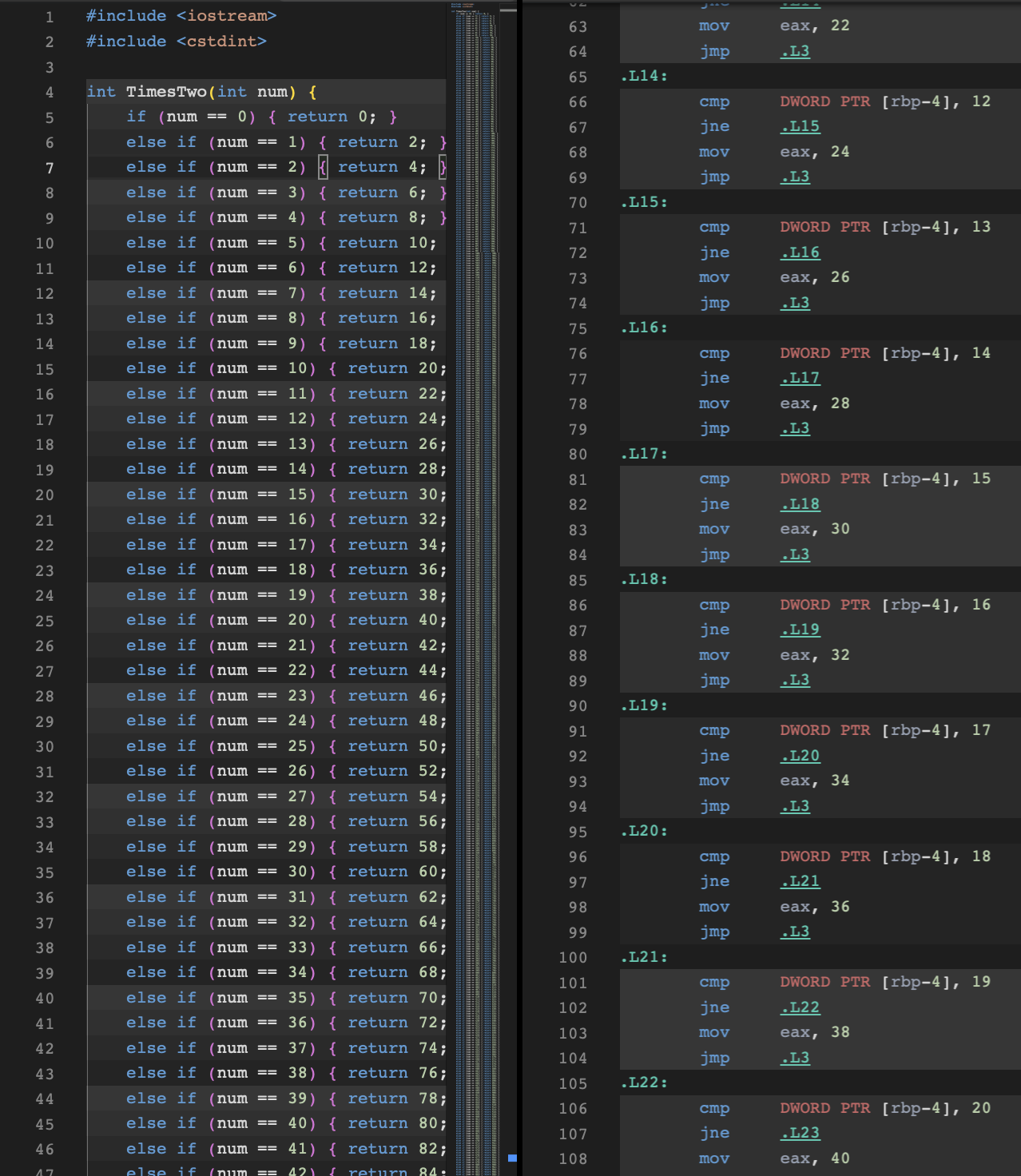
Ideally, each branch would have its own counter to track and predict its outcomes. A real branch predictor is made of a table of many such counters (known in literature as a Pattern History Table, or PHT).
The lower n-bits of the branch’s program counter, or address in memory, are used to index into this table.
 1class BimodalPredictor : public BranchPredictorBase {
 2
 3    ...
 4
 5    std::vector<SatCounter<2>> pred_table;
 6    size_t get_idx(size_t pc) const {
 7        return pc & pc_mask;
 8    }
 9    public:
10
11    ...
12
13        void update(u64 pc, BranchResult branch) override {
14            size_t idx = get_idx(pc);
15            COLLECT_ALIAS(pred_table[idx], pc);
16            pred_table[idx].update(branch);
17            COLLECT_TICK();
18        }
19
20        bool predict(u64 pc) override {
21            return pred_table[get_idx(pc)].predict();
22        }
23    ...
24}
Unfortunately, hardware constraints mean that the PHT is often too small to assign a unique counter to every branch. As a result, one counter may have multiple branches that rely on it for making predictions.
Consider a PHT with 64 entries, and a branch instruction with PC = 87
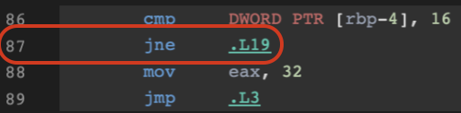
Let’s assign it a counter. 87 in binary is
1010111
The lower 6 bits are:
010111
or 23 in base 10. So, this branch goes into slot 23. There’s a problem though: a branch with PC = 215 (11010111) or PC = 23 (0010111) would also map to this slot, and there’s no way to guard against this.
As you might imagine, this can cause problems like branches overwriting each others’ counters or reading counters trained by conflicting patterns! This aliasing is a real limitation to prediction accuracy, and an engineering challenge that continuously plagues chip designers to this day.
Putting it all together
Now we have a fully-fledged but rudimentary branch predictor. There are 16 slots by default, giving each branch its own dedicated predictor. Try reducing the table size to see what happens:
This type of branch predictor is known as a Bimodal predictor, so-called because it works best when predicting branches that are strongly biased towards either being taken or not taken.
Are we forgetting something?
Taking a step back, we realize two things:
- On its own, a counter can be easily tricked into making terrible predictions
- A single counter remembers very little information about past branch outcomes. A counter trained by 100 successive
TAKENbranch outcomes can be turned to predict the opposite with just twoNOT TAKENs
We can address these concerns by incorporating global branch history into predictions. The process goes as follows:
- We track the outcomes of the past n branches in a data structure called the Global History Register (GHR).
- Take the low n bits of a branch as before, then compute a sort of hash with a slice of the global history. use the result to index into the PHT.
 1template <unsigned hist_len>
 2class HistoryBuffer {
 3    std::bitset<hist_len> history;
 4
 5    public:
 6        HistoryBuffer() :
 7            history(0x0) {}
 8
 9        void update(BranchResult result) {
10            history <<= 1;
11            history.set(0, result);
12        }
13
14    ...
15}
One simple hash we can use is the XOR, or exclusive OR operation, given by this truth table:
| A | B | A XOR B |
|---|---|---|
| 1 | 1 | 0 |
| 1 | 0 | 1 |
| 0 | 1 | 1 |
| 0 | 0 | 0 |
This scheme assigns a separate counter to every combination of a branch and a specific pattern of branch outcomes.
 1class GSharePredictor : public BranchPredictorBase {
 2
 3    ...
 4
 5    std::vector<SatCounter<2>> pred_table;
 6    HistoryBuffer<64> history_buffer;
 7
 8    ...
 9
10    public:
11
12    ...
13
14        u64 get_idx(u32 pc) const {
15            size_t history = history_buffer.as_idx(); // sequence of 1 for taken, 0 for not-taken
16            size_t history_idx = history & history_mask; // chop off bits we don't want
17            return (pc ^ history_idx) & pc_mask; // perform the XOR and trim to table size
18        }
19
20        bool predict(u64 pc) override /*NOT marked const for a very good reason*/{
21            return pred_table[get_idx(pc)].predict();
22        }
23
24        void update(u64 pc, BranchResult branch) override { // update based on resolved branch direction
25            size_t history_idx = history_buffer.as_idx() & history_mask;
26            u64 idx = (pc ^ history_idx) & pc_mask;
27            pred_table[idx].update(branch);
28            history_buffer.update(branch);
29        }
30}
Interactive Gshare:
This is known as a Gshare branch predictor, introduced alongside “Gselect” in a technical note by Scott McFarling.
Anyways, how will this predictor perform in practice? Remember, in a real computer, many branches will be competing for spots in the PHT.
On one hand, incorporating history into our indexing scheme allows for smarter selection. On the other hand, one branch now potentially maps to as many as 2^k different counters, since a sequence of k bits has 2^k possible variations.
Or, you might try convincing yourself that this is actually fine; maybe certain combinations of branch PC and history occur rarely enough that any interference they cause is negligible. These all seem like testable hypotheses…
Evaluating a predictor
Ultimately this thing needs to be printed onto silicon and actually run inside a real computer to be useful. Waiting until you get a physical chip back to validate your branch predictor design is an unacceptably long feedback loop, which is why most companies (and research groups) develop and use elaborate simulators to test their designs.
One such simulation framework is the open-source ChampSim, originally developed to facilitate the Championship Branch Predictor contest. The CBP is a yearly competition where computer architecture research groups publically present new or improved branch prediction algorithms evaluated on various instruction traces gathered from real workloads.
I ran ChampSim on my implementations to test them on 6 different simulated workloads provided by the competition. I collected two different metrics: accuracy (% of correctly predicted branches) and MPKI (Mispredicts Per Kilo-Instruction, the more widely-applicable figure of interest).
Without further ado:
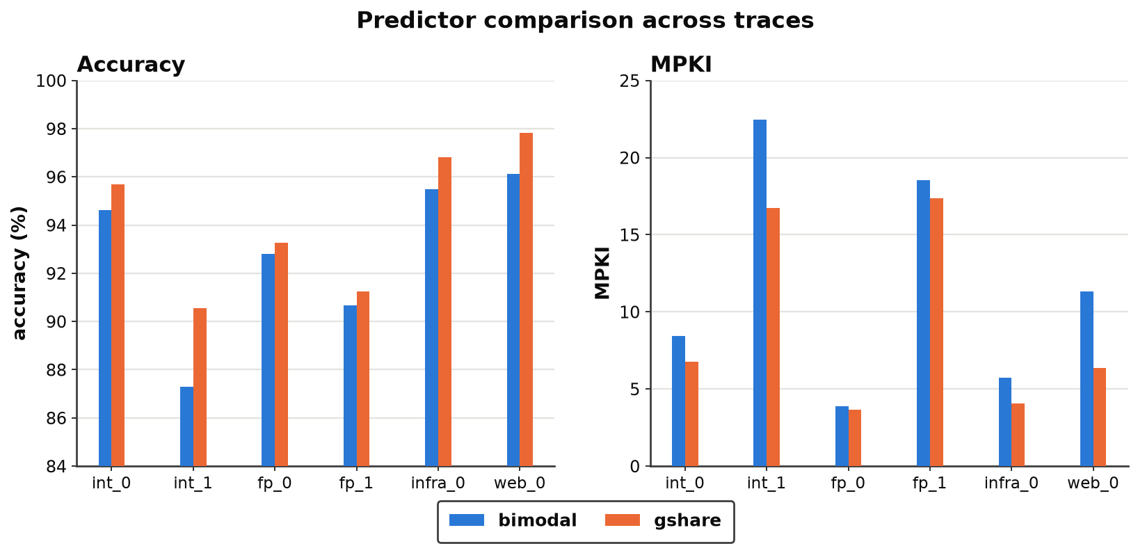
Gshare clearly outperforms bimodal. Very good.
What about our little thought experiment on Gshare storage concerns?
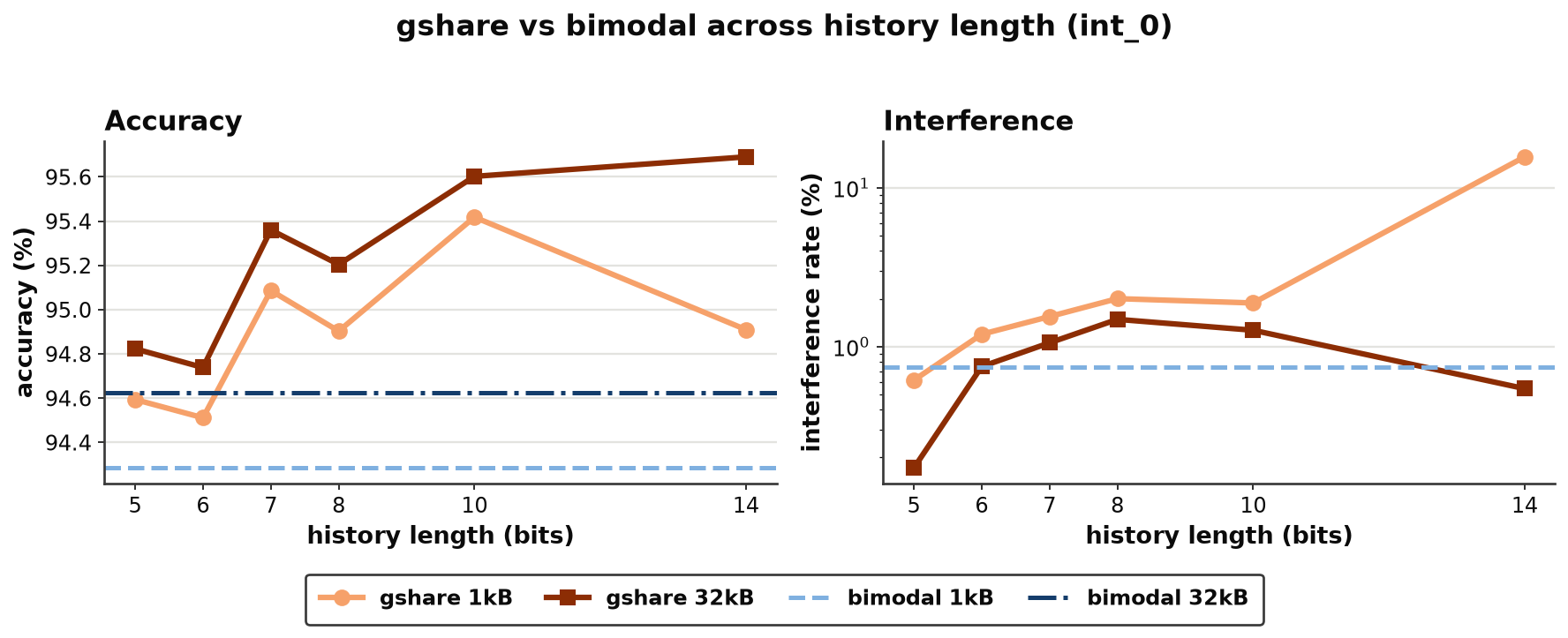
The 1kB / 32kB (more accurately KiB) figure is a measure of much storage a predictor would consume on a real chip.
1kB means we allocate 1024 * 8 / 2 = 4096 2-bit counters
Gshare exhibits a higher overall index collision, just as predicted!
The plot also reveals a clear tradeoff: Increasing history length leads to increased accuracy IF we have enough space. Otherwise, aliasing skyrockets and accuracy drops.
It also may have caught your eye that the accuracy of both bimodal and gshare predictors are already between the high 80%-90% range. This can be attributed to the fact that most branches are actually pretty easy to predict, but have a notoriously long tail of difficulty.
How to build a better branch predictor
Some more observations:
- Taking branch history into account improves accuracy
- There isn’t necessarily a single history length that performs the best
- Performance is sensitive to available storage
These observations have driven much of the research in this area for the past two decades or so.
In 2001, Daniel A. Jimenez and Calvin Lin proposed using a perceptron-based predictor, which uses a weighted sum of history bits to determine a branch outcome. In 2005, Pierre Michaud proposed PPM, which dynamically selects a different history length to use in predictions based on past performance. And in 2006, André Seznec and Michaud proposed TAGE, which became the basis for many modern predictors.
The TAGE branch predictor
TAGE is short for TAgged GEometric history length predictor, which are all certainly words.
The structure of TAGE differs drastically from the previous two designs. Let’s unpack it:
- Instead of a single predictor table, TAGE has multiple, each corresponding to a history length anywhere from 4 to over 1000.
- The history lengths are constructed following a geometrically increasing sequence
- Table entries comprise:
- A 3-bit counter (up from 2) for making predictions
- A tag: metadata for reducing harmful aliasing
- A counter tracking how useful an entry is (referred to as a useful counter)
Additionally, TAGE has a bimodal predictor table to provide “default” predictions. Something like
1class TAGEPredictor : public BranchPredictorBase {
2    ...
3
4    HistoryBuffer<H> _history_buffer;
5    std::vector<SatCounter<2>> _pred_table;
6    std::vector<std::vector<TagEntry<U>>> _banks;
7    ...
Indices and tags are computed via a folded XOR hash which splits the history into equal segments and XORs every segment together along with the low bits of the PC.
Consider this example where we compute a 6-bit index using a 34-bit history:
  older <-------> newer
  h = 1010001001000000100101101110010010

     = 1010 | 001001 | 000000 | 100101 | 101110 | 010010

  001010      h[30:33] (0-padded)
       ⊕ (XOR)
  001001      h[24:29]
       ⊕
  000000      h[18:23]
       ⊕
  100101      h[12:17]
       ⊕
  101110      h[6:11]
       ⊕
  010010      h[0:5]
       ⊕
  111100      PC 0x4A3C & 0b111111
  ______
  100110      index 38 of 64
This is a pretty expensive operation to do from scratch on every prediction. XOR is both associative and commutative, which means the hash can be computed incrementally:
1struct csr { // Circular Shift Register
2    ...
3    void shift_and_fold(BranchResult branch, bool oldest) {
4        u32 out = hash ^ (oldest << cutoff); // remove the oldest history bit
5        out = (out << 1) | (out >> (width)); // left-shift, wrap left-most bit to right-most position
6        out ^= branch; // insert the new history bit
7        hash = out & mask;
8    }
9}
At predict time, the following steps happens in parallel for each table:
- An index i is computed using the folded hash
- A tag t is computed in a similar way
- The entry at index i is read. If the tag stored at that entry matches t, the entry becomes eligible to provide a prediction.
 1bool predict(u64 pc) override {
 2    _top_pred = _pred_table[_get_idx(pc)].predict(); // bimodal predictor
 3    _alt_pred = _top_pred;
 4    _top_idx = -1;
 5    _alt_on_new = false; // fine-tuning technique
 6    for (int i = 0; i < NC; i++) {
 7        u32 idx_hash = _idx_hashes[2*i].hash;
 8        u32 tag_hash = _tag_hashes[2*i+1].hash;
 9        u32 tag_hash_2 = _tag_hashes_2[i].hash; // secondary hash to prevent idx-tag collisions
10
11        u16 idx = idx_hash ^ (pc & _pc_mask);
12        u16 tag = tag_hash ^ (tag_hash_2 << 1) ^ (pc & _tag_mask);
13
14        // this is why predict is non-const
15        _idx_cache[i] = idx;
16        _idx_cache[i+NC] = tag;
17
18        bool pred = _banks[i][idx].predict();
19        bool tag_match = _banks[i][idx].match_tag(tag);
20        if (tag_match) {
21            _alt_pred = _top_pred;
22            _top_pred = pred;
23            _top_idx = i;
24        }
25    }
26
27    ...
28
29    return _top_pred;
30}
The final prediction given by TAGE is the one made by the table corresponding to the longest history length with a matching tag. Also make note of the alternate prediction - the prediction provided by the second longest history table that has a matching tag. In the event of no matching tags, the base bimodal predictor serves as the fallback.
The update step goes as follows:
-
Take the entry that provided the final prediction
-
Increment or decrement the prediction counter depending on branch outcome
-
Update the useful counter
a. Increment the useful counter if the final prediction was correct and different from the alternate prediction
b. Decrement the useful counter if the final prediction was incorrect and different from the alternate prediction
-
Allocate a new entry if the final prediction is incorrect
a. Find the first entry that has a longer history length and has its useful counter set to 0*
b. Overwrite that entry with a fresh set of prediction and useful counters, and the tag computed for the given PC and history length
c. If no such candidate is found, decrement the useful counter of each accessed entry
*This policy varies in literature. Some implementations also check whether the value of the prediction counter is “weak”, that is, straddling the taken/not-taken threshold.
 1void update(u64 pc, BranchResult branch) override {
 2    bool provider_corr = _top_pred == branch;
 3    bool alt_corr = _alt_pred == branch;
 4
 5    if (!provider_corr && !_alt_on_new) {
 6        _allocate_new(branch, pc);
 7    }
 8
 9    ...
10
11    if (_top_idx > -1) {
12        auto pred_idx = _idx_cache[_top_idx]; // reuse previously-computed index
13        _banks[_top_idx][pred_idx].update_ctr(branch); // update prediction counter
14        // update useful counter
15        if (provider_corr && !alt_corr && !_alt_on_new) {
16            _banks[_top_idx][pred_idx].update_u(BranchResult::TAKEN);
17        } else if (!provider_corr && alt_corr && !_alt_on_new) {
18            _banks[_top_idx][pred_idx].update_u(BranchResult::NOT_TAKEN);
19        }
20
21    } else {
22        _pred_table[_get_idx(pc)].update(branch);
23    }
24
25    for (int i = 0; i < NC; i++) {
26        u16 hist_len = _history_lengths[i];
27        bool oldest = _history_buffer.get_bit_at(hist_len-1);
28
29        // update incremental hashes
30        _idx_hashes[2*i].shift_and_fold(branch, oldest);
31        _tag_hashes[2*i+1].shift_and_fold(branch, oldest);
32        _tag_hashes_2[i].shift_and_fold(branch, oldest);
33    }
34
35    _history_buffer.update(branch); // update GHR
36
37    if (_branches_seen++ > 256'000) { // periodically reset useful counters to free up space
38        _reset_all_banks();
39        _branches_seen = 0;
40    }
41}
Each entry now consumes far more space than the modest 2 bits needed in Gshare and bimodal. Every entry now needs to store the prediction counter, the useful counter, and the tag. In return, we get a cache management mechanism that is quite effective at filtering out false matches:
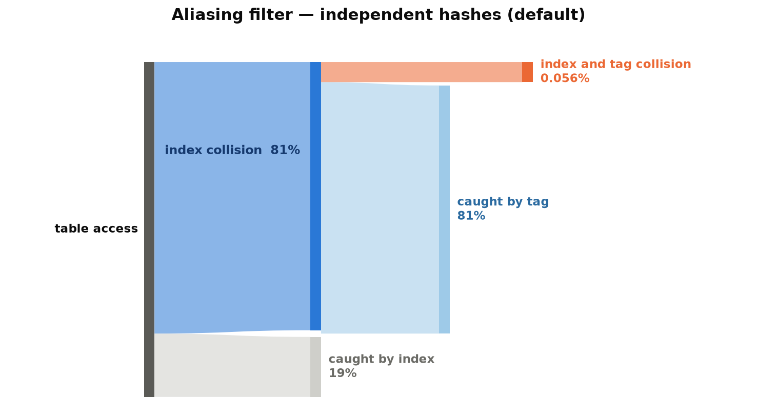
However, one must be careful to keep the tag and index hash functions 1). distinct and 2). uncorrelated:
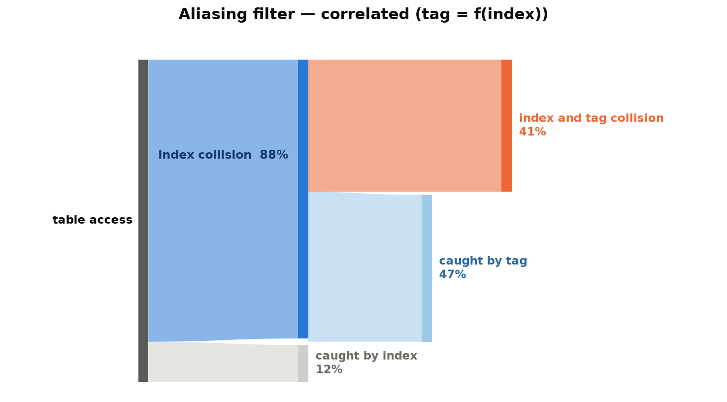
This could happen if, for example, you were to do something like
tag = index 2 * index
How does it compare against the previous two predictors? Overall, a decent improvement across the board except for one workload, fp_0:
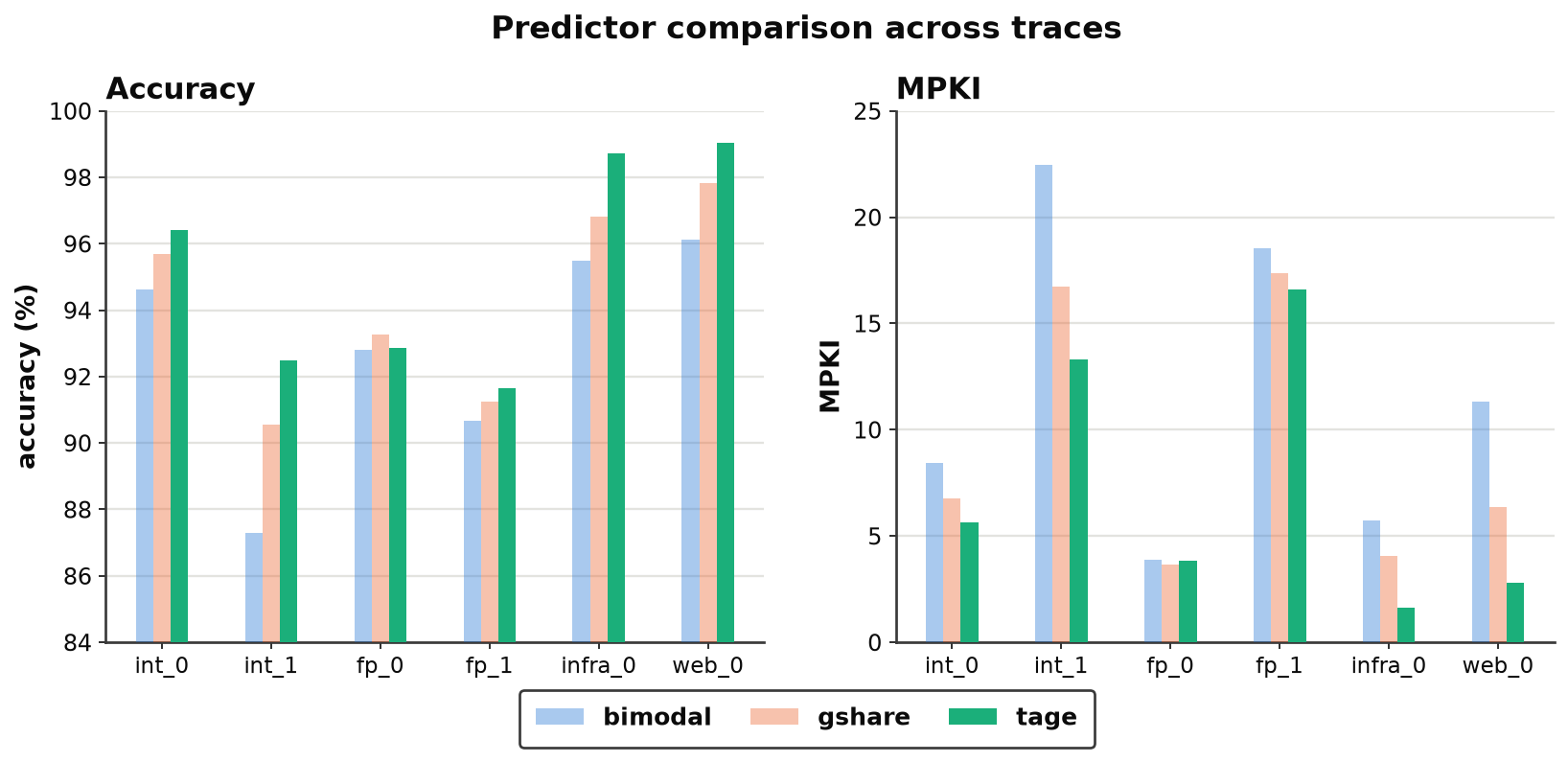
The predictors in this bar graph were each sized to use at most 64kB of simulated hardware storage space in order to standardize comparisons.
The most represented history lengths used in predictions also vary per workload and over time:
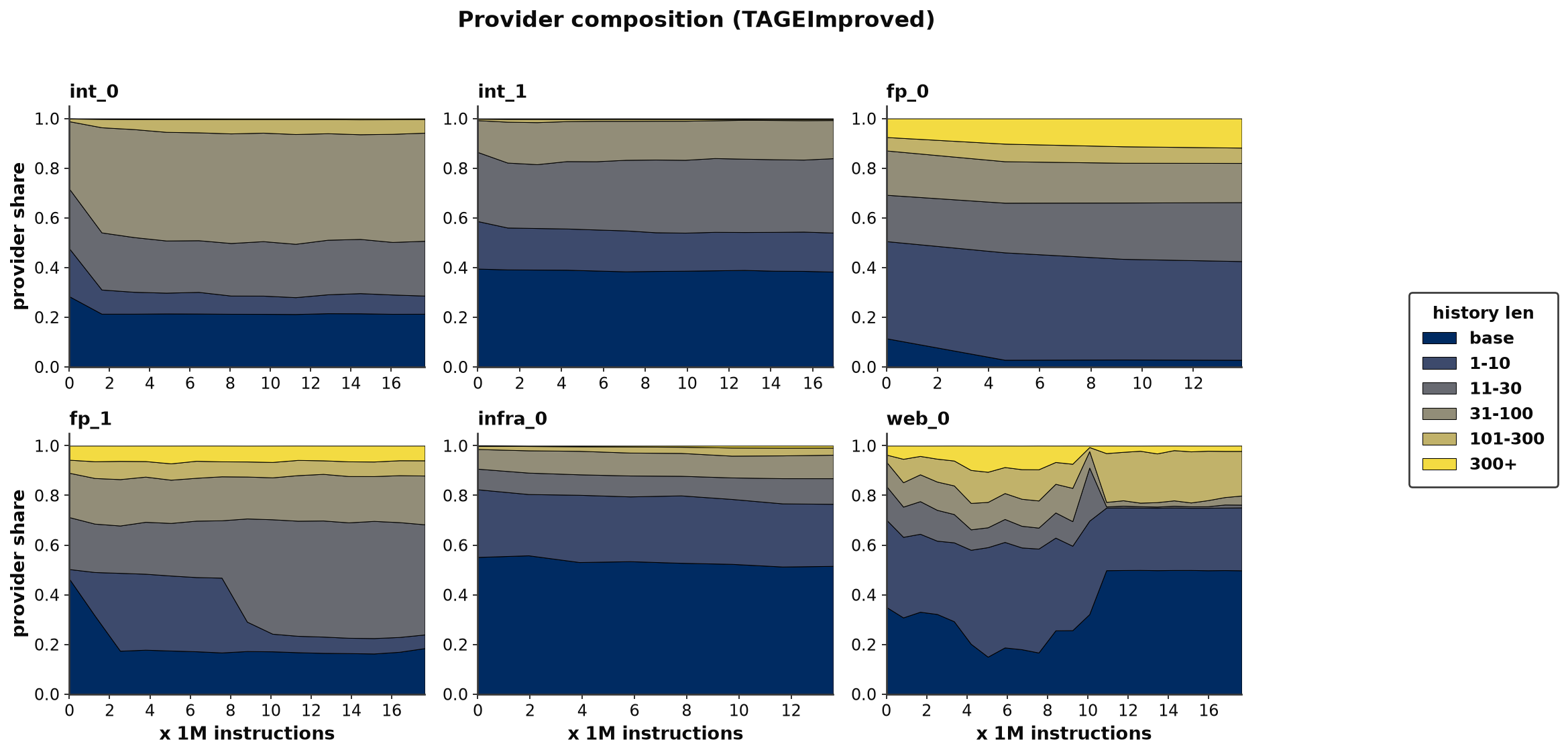
The next plot shows how often the longest history length prediction was correct AND different from the next-longest, weighted by actual prediction count:
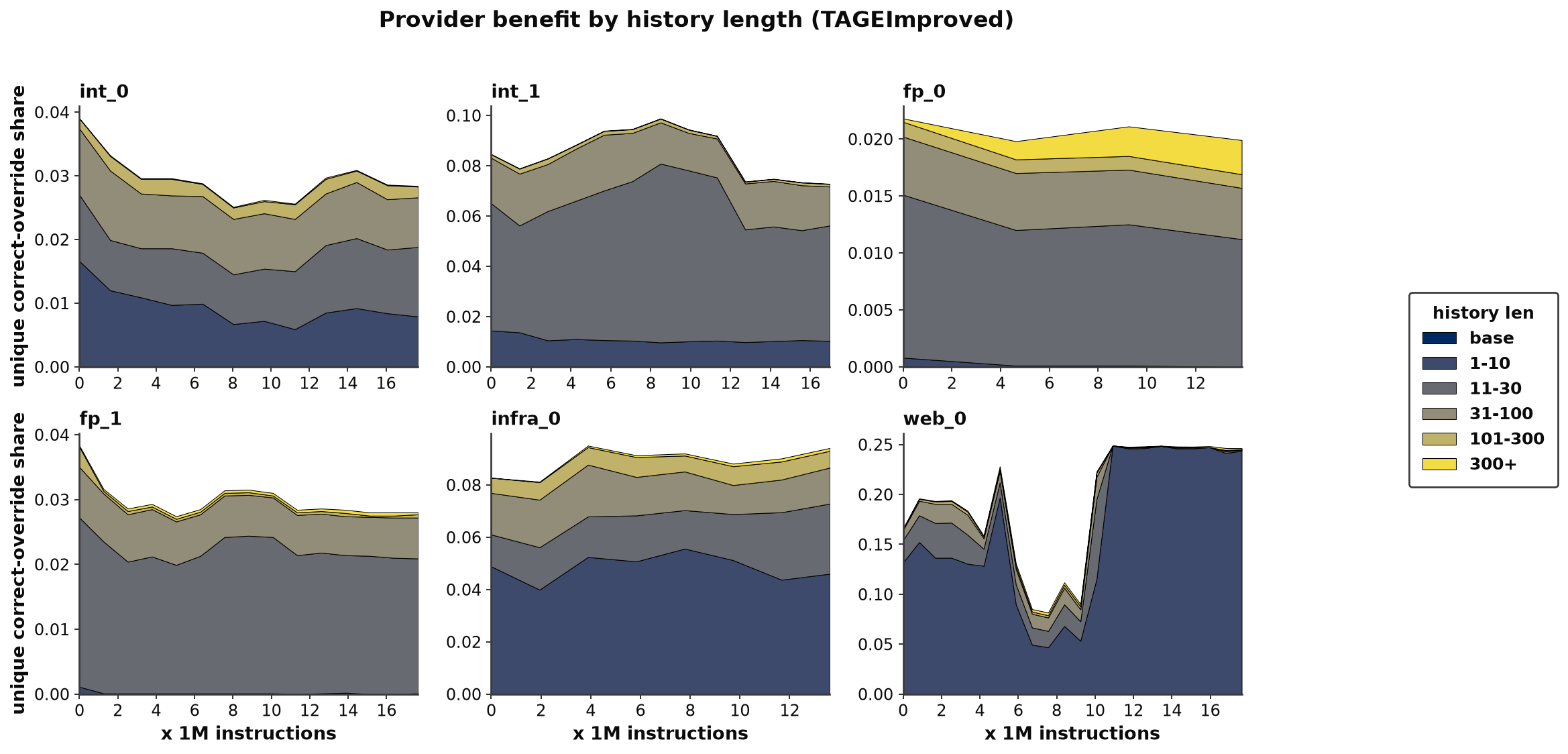
Some observations:
- The trace
fp_0drops in accuracy compared to gshare while also exhibiting a disproportionately higher reliance on long history lengths - The trace
web_0sees a spike in the comparative accuracy of shorter history tables at approximately the same time that the proportion of longer history entries steadily grows- This is followed by a brief period of longer history lengths growing in relative accuracy (between the 7-9 M instruction marks).
- After that, the comparative accuracy of all history lengths past 10 drops significantly despite their overall entry share staying steady.
- This could mean that past a certain program phase, predictions from longer history tables either agree with those from shorter histories or start mispredicting more.
- The fact that TAGE on
web_0yields 50% fewer mispredicts than Gshare makes me lean towards the former.
- A common pattern seen across all provider composition plots is 1). A regime where the history length distribution changes rapidly, followed by 2). a relatively stable steady-state distribution
- This is behavior intrinsic to the structure of the predictor, since it needs to go through many update/predict cycles to learn a pattern across many branches.
- This implies that the typical program sees several discrete “phases” within which the aggregate branching behavior stays relatively stable.
- The overall history table distribution is for the most part dominated by history lengths under 100
- The longest trace shown is about 18 million instructions long. Considering modern processors run in the GHz range, this represents a real-time interval on the order of milliseconds.
By the way, instrumenting branch predictors in this fashion is not a novel practice. My experiments are inspired by this blog post from Karl Mose. It specifically mentions a study that looked at the joint distribution of predictor and useful counters to inform the heuristic behind identifying so-called “cold counters” - counters newly allocated or weakly predicting. The studies in my post are my best guess at other avenues of attack.
Improving on TAGE
The original TAGE design has since undergone many iterations of improvement as described in this paper.
The base TAGE predictor is augmented by two sub-predictors:
- A Statistical Corrector predictor derived from perceptrons to predict branches with a statistical bias
- A “Loop Predictor” specifically designed to detect branch patterns associated with loops
The paper also introduces what it calls “interleaved banks”, which aims to even out utilization across tables by dynamically rotating which predictor table hosts a history length’s entry.
I spent some time reading the associated papers and the original source code to reproduce their results. This took a bit of effort since the algorithms involved were loosely specified in the paper. Specifically, I re-implementented the interleaved banks and statistical corrector.
Interleaved Banks
The standard TAGE implementation always indexes into predictor subbank given a certain history length. However, this turns out not to be ideal because as we saw above, most of the active history lengths are between 1-100.
This means that a large portion of the storage dedicated to the longer history lengths sits unused, while the shorter history are constantly under pressure. The idea behind interleaved banks is to smooth out this asymmetry by rotating the bank assigned to each history length.
Some changes were made to my original implementation. For one, the predictor banks are now just two contiguous vectors. Per-bank indexing is now done by computing the index via folded hash, then adding an offset depending on which bank is being targeted.
 1class TAGEImproved : public BranchPredictorBase {
 2    std::array<std::vector<TagEntry<1>>, 2> _banks = {};
 3
 4    ...
 5
 6    bool predict(u64 pc) override {
 7        ...
 8
 9        u64 t = (shifted_pc ^
10                    (_path_hist & (1 << std::min(27, (int)_history_lengths[_firstLongTagTable])) - 1))
11                % N_L; // compute offset using pc and path history
12
13        for (int i = _firstLongTagTable; i <= nLookups; i++) {
14            if (_noSkip[i]) {
15                _idx_cache[i] += (t << _tage_idx_width);
16                t++;
17                t = t % N_L;
18            }
19        }
20
21    ...
22}
N_L is the number of logical banks used. _path_hist is a new addition too; a hash of previously encountered branch PCs.
Statistical Corrector
The statistical corrector is a linear classifier that sums up counter values across various features, such as global history, path history, the prediction outputted by TAGE, and a fixed bias.
 1class StatCorrector : BranchPredictorBase {
 2    static constexpr u8 CS = 6; // GEHL counter size
 3
 4    static constexpr u8 NUM_BIAS = 2;
 5    static constexpr u8 NUM_GLOBAL_H = 3;
 6    static constexpr u8 NUM_PATH_H = 3;
 7
 8    static constexpr u8 GLOB_H_LEN[NUM_GLOBAL_H] = {10, 40, 64}; // use three global history lengths
 9    static constexpr u8 PATH_H_LEN[NUM_PATH_H] = {24, 16, 9}; // use three path history lengths
10
11    static constexpr u64 tage_weight = 8; // weight given to TAGE prediction
12
13    // bias tables
14    std::vector<SatCounter<CS>> _bias;
15    std::vector<SatCounter<CS>> _bias_sk;
16
17    std::array<std::vector<SatCounter<CS>>, NUM_GLOBAL_H> _w_global; // table with global history counters
18    std::array<std::vector<SatCounter<CS>>,NUM_PATH_H> _w_path_hist; // table with local history counters
19
20    ...
21
22}
Note that each counter now has 6 bits!
Each of these tables are each indexed using a fancy hash combining the prediction given by TAGE, the global/path history, and of course, branch PC.
1u64 _get_gh_idx(u64 pc, int i) { // global history indexer
2    return ( (pc >> 2) ^ _gh_hashes[i].hash ^ (_tage_pred << 9) ) & _global_hist_mask;
3}
Putting it all together…
 1bool predict_sc(u64 pc) {
 2    u64 tage_contrib = tage_weight * _last_tage_ctr;
 3
 4    u64 midpoint = num_tables * SatCounter<CS>::midpoint() + tage_weight * SatCounter<3>::midpoint();
 5    u64 threshold = _get_threshold(pc);
 6
 7    // sum together all "features"
 8    u64 sum = 0;
 9    sum += _get_bias(pc);
10    sum += _get_gh_prediction(pc);
11    sum += _get_path_prediction(pc);
12    sum += tage_contrib;
13    _last_sum = sum;
14    _sc_pred = sum >= midpoint;
15    int midpoint_distance = std::abs((int)_last_sum - (int)midpoint);
16    bool override_tage = (_sc_pred != _tage_pred) & (midpoint_distance > threshold);
17
18    // override TAGE prediction by default
19    // if TAGE is high-confidence, sometimes preserve TAGE
20    if (_sc_pred != _tage_pred) {
21        if (_tage_conf.high_conf) {
22            if ((midpoint_distance < threshold / 2) & (midpoint_distance >= threshold/4)) {
23                override_tage = !_lc_chooser.predict(); // large counter determines override or not
24            }
25        }
26    }
27    _last_pred = override_tage ? _sc_pred : _tage_pred;
28
29    return _last_pred;
30}
The prediction outputted by the statistical corrector gives the final call on which direction to predict.
Was it worth it?
The improvements were marginal but visible:
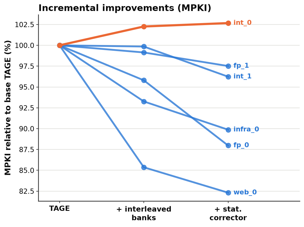
This iteration fails to improve on trace int_0.
The full details can be found on my GitHub repo (repro steps coming soon).
Here’s how it compares overall:
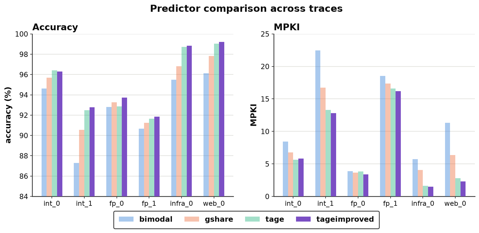
Interestingly, “tageimproved” now beats out all previous predictors on fp_0.
Finally, I compared how my implementation did against a reference implementation written by the inventor of TAGE:
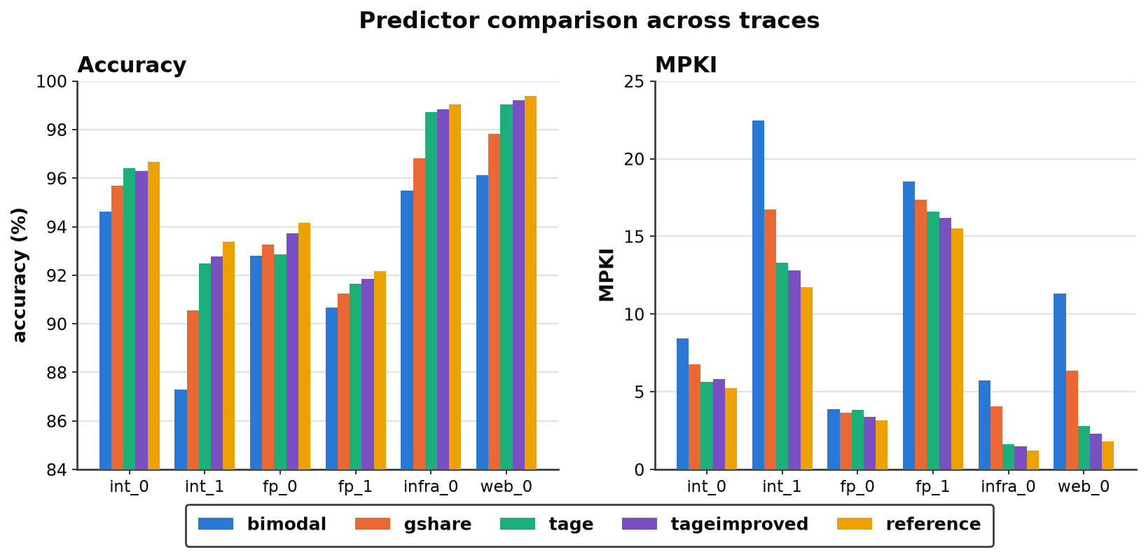
It wins out across the board.
Is it impressive that my implementation scores so closely? Not really, for a couple reasons:
- Like I mentioned before, my “tageimproved” variant was based largely on the reference implementation
- The gap between 98% and 100% is extremely hard to close. Reasons for this include sparsely encountered branches (limited opportunity to train the predictor), stochastic variations (impossible to extract a signal by construction), or patterns outright too complicated for existing algorithms.
Great, let’s see the hardware implementation
(Disclaimer: I am NOT a hardware engineer. If I've missed anything and you have opinions, please reach out!)
Unfortunately, a branch predictor with the features described above is impractical for actual hardware due to latency, area, and power requirements, as conceded by the authors of TAGE. Many early publications (2008 - ca. 2020) describe designs optimized specifically for performance on the ChampSim simulator.
In 2024, Seznec released a whitepaper detailing a modified version of his predictor that would actually be feasible to implement in real hardware. No more local per-branch history tracking, no more extensive history bank interleaving. This new design (perhaps unsurprisingly) performed slightly worse than the 2016 version.
Despite it all, there is strong evidence that most modern processors use a branch predictor design inspired by or derived from that of TAGE.
I think the most remarkable fact here is that the folded XOR hash function does a decent job of capturing patterns across such a wide range of branch histories.
If we had infinite storage and infinite time to make a prediction, the useful counter and tag mechanism become unnecessary. Even folding histories would become unnecessary, since we could just use some fancy hash function with much better collision guarantees to generate a unique index for every (PC, history) pair.
But unfortunately, chip area is finite, and predictions must be provided within a few clock cycles to keep the processor smoothly running. All the tricks described above are the consequences of the intense selective pressure of this low-latency low-storage environment.
Final thoughts
Writing, debugging, and evaluating these virtual branch predictors was a uniquely challenging experience. LLMs served as a last resort when I hit a dead end, but I was determined to hand-write as much of this as I could. I will, however, shamelessly admit that I had Claude write pretty much everything to do with data plumbing and visualization.
Sometimes, a bug would give comically bad results. Other times, I’d get subtly wrong results: a slight regression, unsatisfactory accuracy, etc. I couldn’t just print out every branch and its effect on the internal state of my predictor; on a million+ instruction trace this would be absurd. So, I had to get a bit clever to extract the most actionable information per request to std::ostream& os operator<<. This eventually led to the idea of actually presenting this data as a standalone method of interpreting the internals of a branch predictor. I’m curious about other instances where diagnostic information was repurposed in this manner.
Most of the state-of-the-art implementations that I encountered are also a prime example of “the code is the spec”. The publications introducing these implementations provided what mostly amounted to an outline, with the algorithm’s details available only through reading the (at-times cryptic) code. Reconciling the high-level descriptions given in the papers with the nitty-gritty implementation details was nonetheless enlightening.
At the beginning of this post I feigned incredulity at the fact that modern branch predictors are:
- are correct over 98% of the time
- are essentially small neural networks embedded in the chip
- look hundreds or even thousands of branches into the past to make decisions
Well, it turns out that these are all true in some way or another! Pretty cool considering that these hardware structures need to run with subnanosecond delay. Appropos of that…
All the plots and code snippets can make it easy to forget that these algorithms must be implemented as digital circuits. These designs are embedded in silicon and running constantly in your phone and computer RIGHT NOW!! Isn’t that crazy?